CSC2515 :: Machine Learning :: Final Project
On Learning Surface Light Fields
You can download a pdf version of the paper here.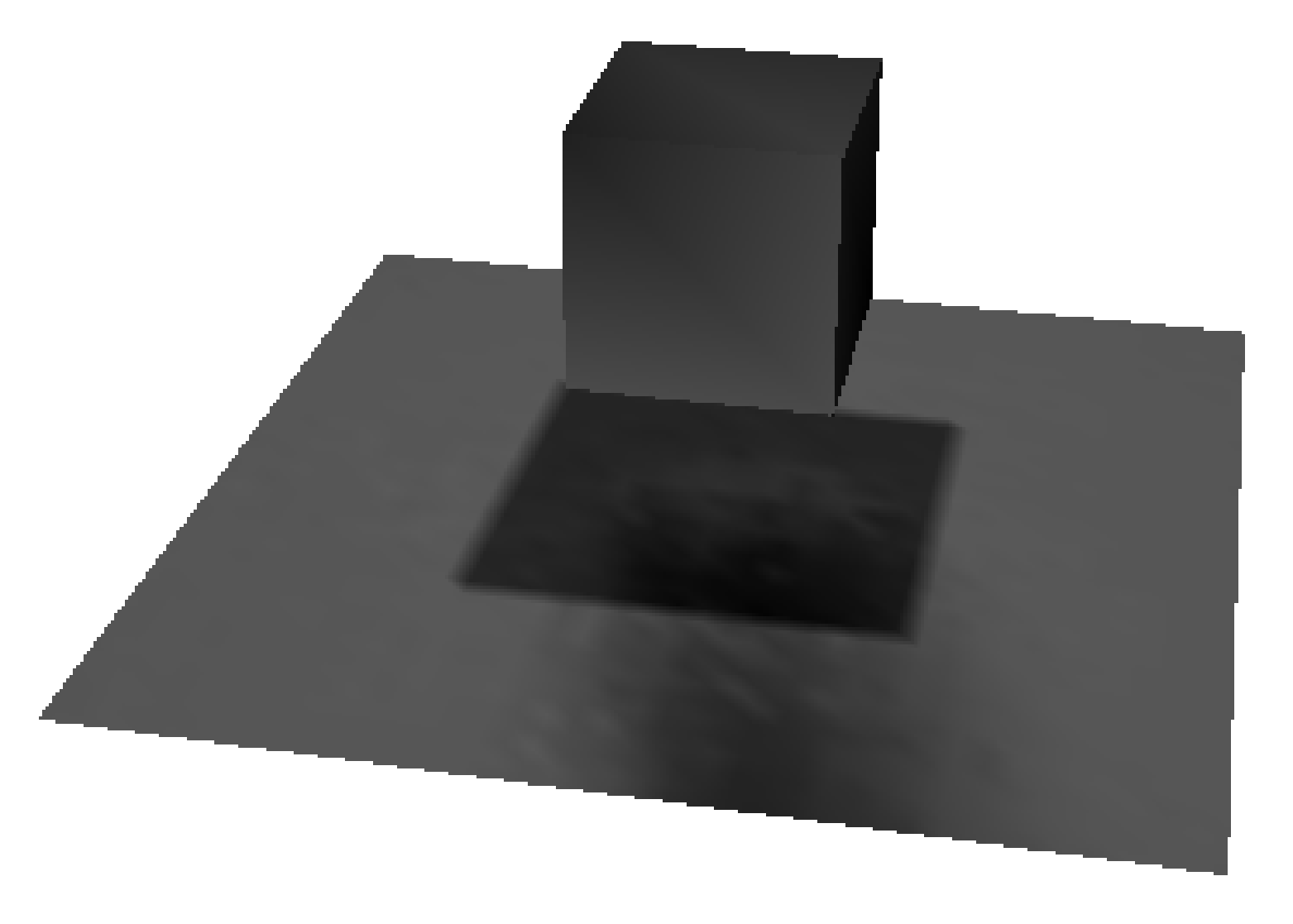 |
 |
 |
| Table 1: Estimated color values for GBF (left) and VMBF (right) and correct image for a scene with high-frequency effects. The average error rates over all vertices are 0.0302 for the GBF and 0.0322 for the VMBF. | ||
Introduction
The five-dimensional surface light field function
[Miller 1998]
represents the exitant radiance for all surface points in a scene. Its
value incorporates all light transport effects such as shadows,
reflection and refraction. In the past, tabulated or re-sampled color
values [Miller 1998] [Wood 2000]
have been used to approximate the surface light field function and the
exitant radiance for new views has been interpolated from the stored
values.
We propose the use of a radial basis function (RBF) network to
approximate the surface light field. The parameters of the RBF network
are obtained by supervised learning. At runtime these parameters are
used to generate the exitant radiance for surface points for previously
unknown view directions. The von Mises function
[Arnold 1941]
is employed as basis function for the RBF network. It is particularly
well suited for the given problem as it is defined on the surface of
the sphere which is the domain of the surface light field function. In
the past, Gaussian basis functions have been used to approximate view
depend functions [Green
2006]
but such functions defined in Cartesian space suffer from the artifacts
well known from cartography when mapping the surface of the earth onto
a planar map; e.g. the distortion near the poles and the loss of the
periodicity on the sphere.
In this work, we implemented an radial basis function network with
von Mises basis functions (VMBF) to evaluate the suitability of this
architecture for approximating surface light fields. An RBF network
with Gaussian basis functions (GBF) has been implemented for comparison
purpose. Our results show that, for a small number of basis functions,
the VMBF outperforms the GBF but for 16 and more basis functions the
GBF is superior. However, our results are limited in that only two
scenes have been examined and, therefore, general conclusions are
hardly possible.
Related Work
Related work to our approach can be found in the Machine
Learning and the Computer Graphics literature.
In Computer Graphics, surface light fields, which are an image-based
rendering techniques (IBR), and precomputed radiance transfer (PRT) are
similar to our approach. Surface light fields have been introduced by
Miller et al. [Miller 1998] who adapted the lumigraph [Gortler
1996] but only represented the light field on the surface of
the scene objects. Wood et al. [Wood
2000]
extended this approach and used least-squares optimal lumispheres,
subdivided octahedron whose vertices are used as directional samples,
on a dense but discrete set of surface sample points to approximate the
surface light field. The color values at the sample points have been
obtained using learning techniques and compressions schemes such as
function quantization and principal function analysis; generalizations
of vector quantization and principal component analysis, respectively;
are used to obtain the necessary reduction of the storage size. Zickler
et al. [Zickler 2005]
trained a combination of lower-order polynomials and locally weighted
regression to approximate a surface light field. Their model uses every
visible surface point as training sample but they reported that, in
practice, only a subset of these points is used to reduce the
computational complexity. This is similar to our work.
PRT differs from these techniques and our approach in that
transferred and not exitant radiance is stored. This permits to change
the lighting environment at runtime but, in contrast to our work,
prohibits local light sources. Most PRT techniques approximate
transferred radiance by projecting the information into a set of basis
functions so that only the coefficients have to be stored, which
reduces the memory requirements significantly. A similarity with our
work is the use of spherical basis functions, e.g. Spherical Harmonics
[MacRobert 1948].
In fact, this work motivated us to explore the VMBF to approximate
surface light fields. Recently, Green et al. [Green 2006]
used machine learning techniques to approximate transferred radiance
for high-frequency, view-dependent effects such as specular highlights.
They employed a Gaussian mixture model which, compared to previous
techniques, reduced the necessary number of coefficients significantly.
In this work a semi-parametric model is used, training one RBF network
for each view direction of each vertex. Our approach is similar to
[Green 2006]
in that the same RBF architecture is employed but differs from their
work as we train only one RBF network per vertex, each approximating
the information for all view directions.
Besides the vast amount of work on radial basis functions in general
(see [Bishop 1995]
for a good introduction to RBF networks), there is only little related
work on problems defined on the surface of the sphere in the Machine
Learning community. The most relevant one is those by Jenison and
Fissel [Jenison 1995]
[Jenison 1996].
In [Jenison 1995]
the superiority of the VMBF over the GBF for the problem examined in
this paper is demonstrated. [Jenison
1996] applies the VMBF to an regression problem defined on
the surface of the sphere.
Model Specification
Approximating the surface light field is a regression problem. In this section the proposed model to learn this function is introduced.Von Mised Basis Functions
The VMBF is based on the Mises-Arnold-Fisher distribution [Arnold 1941], a spherical probability density function (pdf) which is the equivalent to the normal distribution [Fisher 1987] on the surface of the unit sphere. The normalization factor of the pdf can be absorbed into the weights of the RBF network ([Bishop 1995], p. 168) which yields the following basis function

where ![]() and
and ![]() are the function arguments in spherical polar coordinates for azimuth
and elevation, respectively,
are the function arguments in spherical polar coordinates for azimuth
and elevation, respectively, ![]() and
and ![]() determine the center of the function on the surface of the unit sphere
and
determine the center of the function on the surface of the unit sphere
and ![]() is a concentration parameter which determines the function width. Using
such a function defined on the sphere is desirable as this naturally
enforces the periodicity of the spherical domain and the singularity at
the poles. A detailed introduction and a discussion of the properties
of this function can be found in [Fisher
1987].
is a concentration parameter which determines the function width. Using
such a function defined on the sphere is desirable as this naturally
enforces the periodicity of the spherical domain and the singularity at
the poles. A detailed introduction and a discussion of the properties
of this function can be found in [Fisher
1987].
Gaussian Basis Functions
The well known Gaussian basis function is used for comparison purpose. First, because it is the standard basis functions for RBF networks ([Bishop 1995], p. 165) and second because it has been used in related work [Green 2006]. As for the VMBF, the normalization factor of the GBF can be absorbed into the weights of the RBF network. Following [Green 2006] we use a spherical covariance matrix which yields
where ![]() is
the argument of the function,
is
the argument of the function, ![]() is the two-dimensional center of the Gaussian and
is the two-dimensional center of the Gaussian and ![]() is its variance.
is its variance.
Radial Basis Function Network
The Radial Basis Function network is given by
where ![]() is the
is the ![]() -th
basis function and
-th
basis function and ![]() is its weight. All basis functions are considered as independent, i.e.
no parameters are shared. This architecture can also be interpreted as
a generalized linear model.
is its weight. All basis functions are considered as independent, i.e.
no parameters are shared. This architecture can also be interpreted as
a generalized linear model.
Methodology
The surface light field is a five-dimensional function;
three
dimensions determine a position in space and two the direction of the
exitant radiance in spherical polar coordinates. Following previous
work [Wood 2000],
we tabulate the spatial domain at each vertex and learn the
view-dependent exitant radiance for each surface sample using an RBF
network. For the VMBF, this yields a model with ![]() parameter,
where the first term in the sum models the number of
parameters for the non-normalized von Mises basis functions and the
weights for each of those,
parameter,
where the first term in the sum models the number of
parameters for the non-normalized von Mises basis functions and the
weights for each of those, ![]() is the number of basis functions employed for sample
is the number of basis functions employed for sample ![]() and
and ![]() is the total number of vertices. The tabulated surface samples are
treated as independent which simplifies the training significantly
because in this case only
is the total number of vertices. The tabulated surface samples are
treated as independent which simplifies the training significantly
because in this case only ![]() parameters
have to be optimized simultaneously. However, each
optimization still remains non-trivial as determining the parameter for
an RBF network is a nonlinear and non-convex problem ([Hastie 2001],
page
36).
parameters
have to be optimized simultaneously. However, each
optimization still remains non-trivial as determining the parameter for
an RBF network is a nonlinear and non-convex problem ([Hastie 2001],
page
36).
We employ numerical optimization to find parameters which minimize the
sum of squared errors, the error function used in this work. Weight
decay is used to regularize the optimization and avoid overfitting
([Hastie 2001], p.
356). The objective function is therefore given by
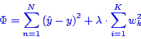
where ![]() is the estimated function value and
is the estimated function value and ![]() is its true value. The second term is the weight decay, where
is its true value. The second term is the weight decay, where ![]() is a tuning parameter. The training set consists of color value-view
direction pairs.
Due to the periodicity of the sphere, no constraints on
is a tuning parameter. The training set consists of color value-view
direction pairs.
Due to the periodicity of the sphere, no constraints on ![]() ,
,
![]() and
and
![]() are
necessary for the VMBF. For the GBF, the variance has to be
positive. We enforce this by computing the gradient w.r.t.
are
necessary for the VMBF. For the GBF, the variance has to be
positive. We enforce this by computing the gradient w.r.t. ![]() in
the learning phase.
in
the learning phase.
The gradients of the objective function, which are necessary for the
numerical optimization, can be derived using the chain rule and found
in [Jenison 1996]
for the VMBF and in text books for statistics for the GBF.
Implementation
The learning procedure described in the previous section
has been
implemented in Matlab and C++. The training data has been generated
using Mental Ray, a commercial high-quality renderer. The particular
choice has been made because the Mental Ray integration in Maya allows
to directly store vertex colors from pre-rendered scenes. We also
experimented with generating images and extracting the color values
using image processing techniques. However, in our tests this approach
was highly error prone. The view directions are randomly drawn from the
set of all possible view directions, for our test scenes in the upper
hemisphere above the scene origin. Stratified sampling has been used to
reduce the variance of the sample directions [Veach 1997].
One of the main issues which arose during the implementation were the
long optimization times. To reduce these, only monochrome surface light
fields have been examined this report. In general, different wavelength
of light can be considered as independent, so that the results obtained
can be generalized for images with multiple color channels. Other
strategies to reduce the amount of computations are discussed in the
next section.
The vertex color for a new images can be obtained by evaluating the RBF
architecture for a particular view direction ![]() with the parameters found in the training phase. Given the estimated
vertex color values, the model can be rendered using standard renderer.
Our current implementation uses Maya for this.
with the parameters found in the training phase. Given the estimated
vertex color values, the model can be rendered using standard renderer.
Our current implementation uses Maya for this.
Results
Increasing ![]() reduces the test error rate but the decrease shows an asymptotic
behavior, so that, beyond a certain point, the error can not be lowered
significantly by using more training data. This makes it possible to
bound the training set size without degrading the quality. For most
problems also an optimum for the model complexity, this is the number
of basis functions for an RBF network, exists. Next to these two
parameter, also an optimal value for the weight decay tuning parameter
reduces the test error rate but the decrease shows an asymptotic
behavior, so that, beyond a certain point, the error can not be lowered
significantly by using more training data. This makes it possible to
bound the training set size without degrading the quality. For most
problems also an optimum for the model complexity, this is the number
of basis functions for an RBF network, exists. Next to these two
parameter, also an optimal value for the weight decay tuning parameter ![]() had to be found.
had to be found.
A particular difficulty was that different optimal values ![]() ,
,
![]() and
and
![]() might
exist for each vertex; so essentially we were faced with
might
exist for each vertex; so essentially we were faced with ![]() regression problems instead of one. However, using
regression problems instead of one. However, using ![]() different sets of optimal parameters is not tractable. First, because a
full cross-validation over the three dimensional parameter space would
be necessary for each vertex; this was prevented by the long
optimization times; and second, because using different parameters
would prohibit an efficient implementation of the re-rendering.
different sets of optimal parameters is not tractable. First, because a
full cross-validation over the three dimensional parameter space would
be necessary for each vertex; this was prevented by the long
optimization times; and second, because using different parameters
would prohibit an efficient implementation of the re-rendering.
Next to the already mentioned restriction to monochrome images, further
simplification were necessary to reduce the computational complexity
and obtain the results of the exploration in a reasonable time. We used
only a randomly generated subset of the vertices for the experiments to
achieve this.
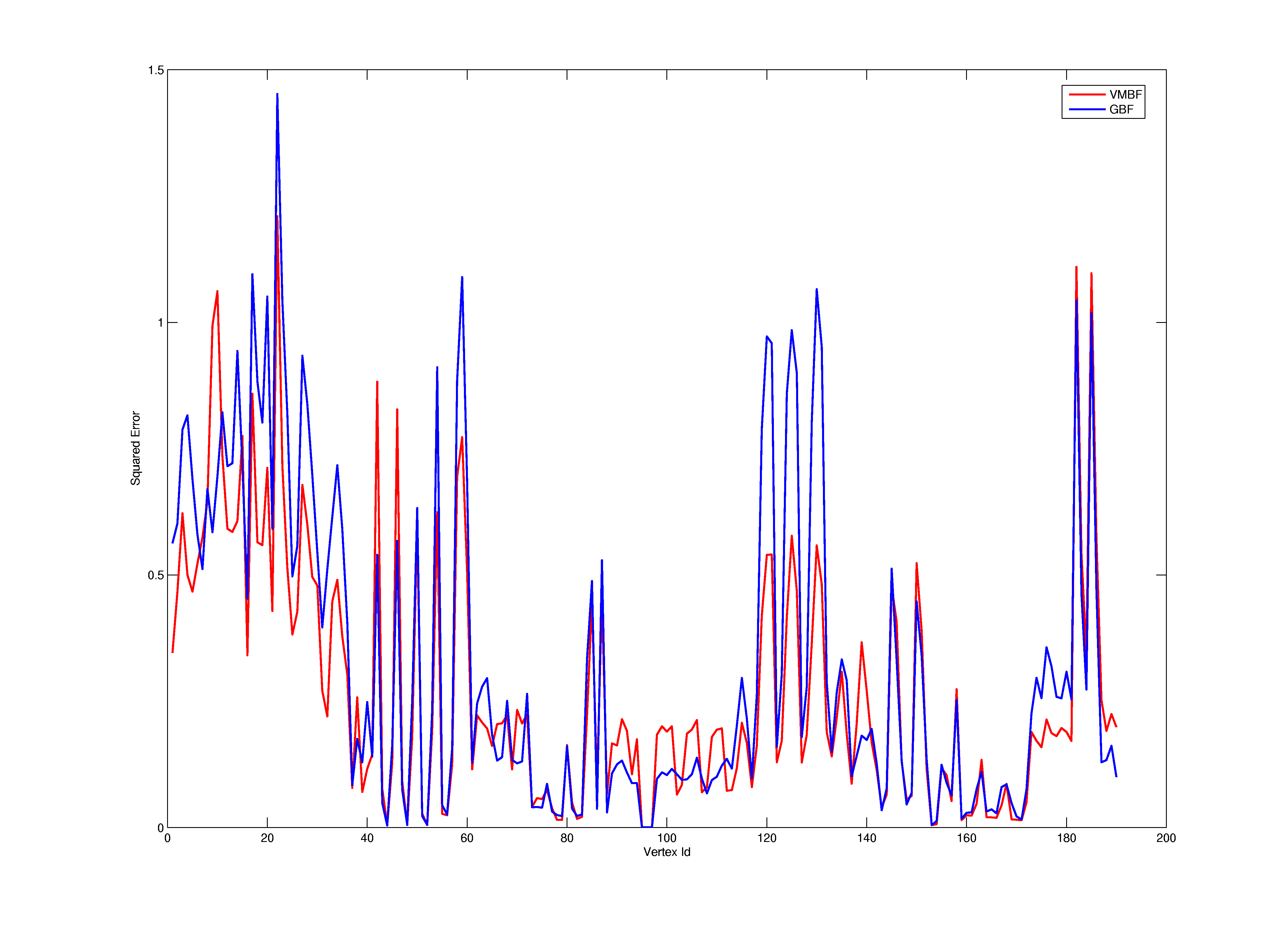
The test scenes employed in our experiments contained 1689 (Table 1)
and 190 vertices (Table 4); 16 and 17 vertices have been used for the
exploration of the hyperparameter space, respectively. The
three-dimensional search space was spanned by ![]() ,
, ![]() and
and ![]() .
.
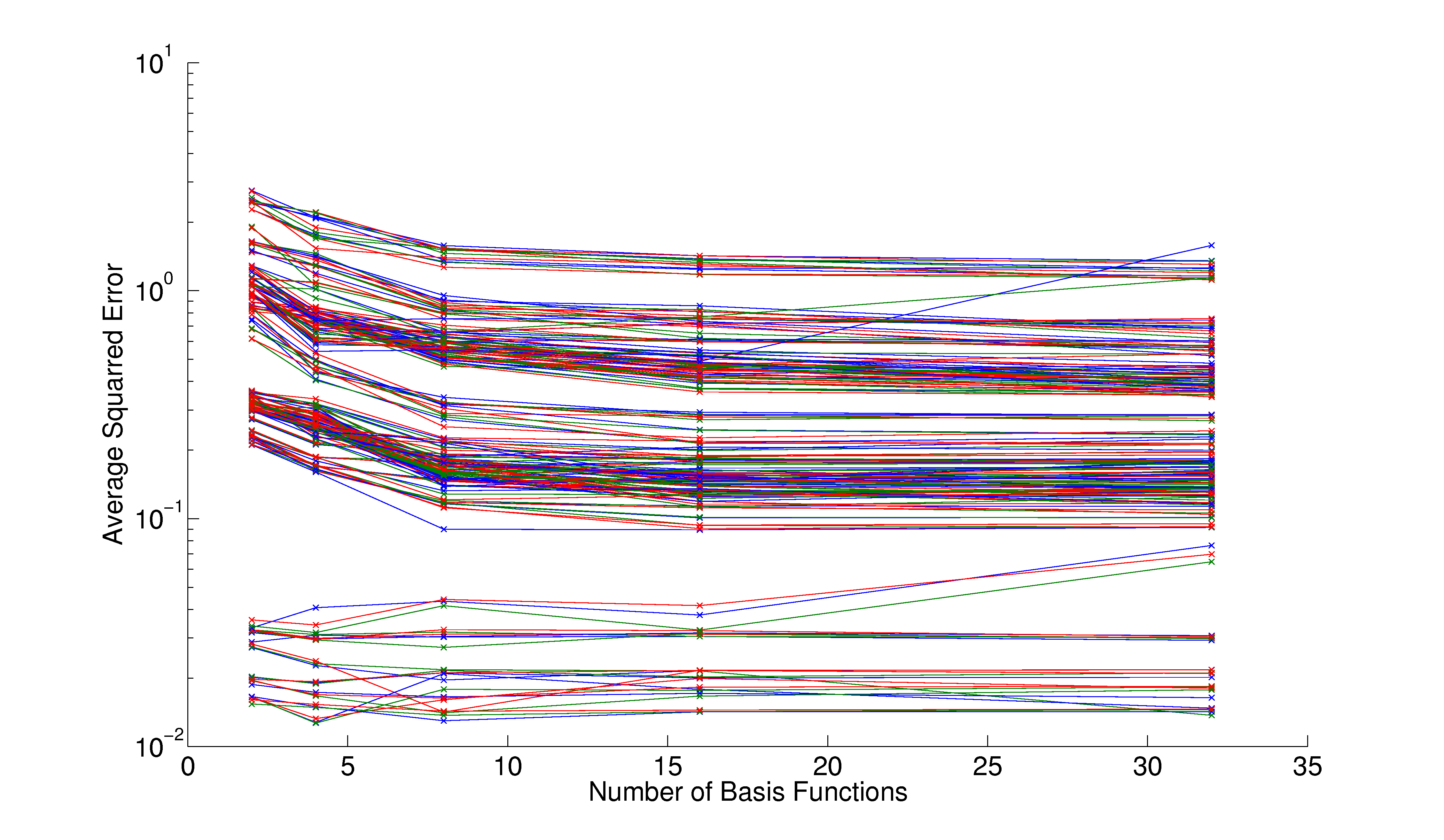
The sum of the error rates over all vertices on a test
set of size 200
for the VMBF and the GBF are shown in Table 2 and Table 3. It can be
seen that all graphs show an asymptotic behavior for increasing values
of ![]() .
In Table 3, this behavior is more significant whereas the error rates
in Table 2 decrease over the whole range of
.
In Table 3, this behavior is more significant whereas the error rates
in Table 2 decrease over the whole range of ![]() .
Unfortunately, no optimum for
.
Unfortunately, no optimum for ![]() exist. For the VMBF, values of 8 or 16 for
exist. For the VMBF, values of 8 or 16 for ![]() are sufficient as the error does not decrease substantially for higher
values; however, for the GBF such a close-to-optimal value of
are sufficient as the error does not decrease substantially for higher
values; however, for the GBF such a close-to-optimal value of ![]() does not exist. Table 2 and Table 3 also show that, for different
values of the ridge regression tuning parameter
does not exist. Table 2 and Table 3 also show that, for different
values of the ridge regression tuning parameter ![]() ,
the error rates do not differ significantly. In contrast to this, for
both basis functions the error rates for 200 views are higher than
those for 500. For the VMBF, a training set size of 500 is sufficient
to achieve an almost optimal error rate. This also holds for the GBF
for the scene with 1689 vertices (Table 3). For the results reported in
Table 2, this close-to-optimal value is reached for 750 views for the
GBF. The graphs in Table 2 show that the error rates for 1000 views are
higher than those for 750 views. We assume the reason for this is the
non-convexity of the optimization.
,
the error rates do not differ significantly. In contrast to this, for
both basis functions the error rates for 200 views are higher than
those for 500. For the VMBF, a training set size of 500 is sufficient
to achieve an almost optimal error rate. This also holds for the GBF
for the scene with 1689 vertices (Table 3). For the results reported in
Table 2, this close-to-optimal value is reached for 750 views for the
GBF. The graphs in Table 2 show that the error rates for 1000 views are
higher than those for 750 views. We assume the reason for this is the
non-convexity of the optimization.
In both scenes, for ![]() the GBF achieves lower error than the VMBF. For
the GBF achieves lower error than the VMBF. For ![]() the error rates are roughly equivalent and for lower values of
the error rates are roughly equivalent and for lower values of ![]() the VMBF outperforms the GBF. The error rates for
the VMBF outperforms the GBF. The error rates for ![]() are not reported in Table 2 and Table 3 but here, the error rates for
the GBF are an order of magnitude higher than those for the VMBF. An
interesting observation is that, for the VMBF, the vertices clearly
form clusters w.r.t. to the error rates; a behavior which does not
exist for the GBF.
A comparison of the error rates of the two scenes shows that those
reported in Table 3 are significantly below those in Table 2. This is
surprising as both scene have almost the same materials and lighting
environment; the only main difference is the spatial resolution of the
sample points. In this section, the results obtained during the
exploration of the
hyperparameter space are discussed. The goal of the experiments was to
find a number of basis functions
are not reported in Table 2 and Table 3 but here, the error rates for
the GBF are an order of magnitude higher than those for the VMBF. An
interesting observation is that, for the VMBF, the vertices clearly
form clusters w.r.t. to the error rates; a behavior which does not
exist for the GBF.
A comparison of the error rates of the two scenes shows that those
reported in Table 3 are significantly below those in Table 2. This is
surprising as both scene have almost the same materials and lighting
environment; the only main difference is the spatial resolution of the
sample points. In this section, the results obtained during the
exploration of the
hyperparameter space are discussed. The goal of the experiments was to
find a number of basis functions ![]() and the training set size
and the training set size ![]() which provide efficient pre-computation as well as accurate
re-rendering. For an efficient pre-computation, both,
which provide efficient pre-computation as well as accurate
re-rendering. For an efficient pre-computation, both, ![]() and
and ![]() ,
should be as small as possible. However, this conflicts with the
desired accuracy.
,
should be as small as possible. However, this conflicts with the
desired accuracy.
Using the results obtained through the exploration of
the
hyperparameter space, we trained an RBF networks with the VMBF and the
GBF with a training set of size 500, ![]() and
and ![]() for both of our test scenes. The parameters have been chosen based on
the optimal values for the VMBF. Here, we decided to use
for both of our test scenes. The parameters have been chosen based on
the optimal values for the VMBF. Here, we decided to use ![]() instead of
instead of ![]() because the error rates do not differ significantly but the
optimization time is much higher for
because the error rates do not differ significantly but the
optimization time is much higher for ![]() .
In terms of re-rendering,
.
In terms of re-rendering, ![]() is also a better choice for the experiments as it is an upper limit for
an efficient implementation of the re-rendering on the GPU.
is also a better choice for the experiments as it is an upper limit for
an efficient implementation of the re-rendering on the GPU.
The results for one view of the test set for the scene with 1690
vertices can be seen in the images in Table 1. For the chosen parameter
values, both basis functions are not capable of capturing the hard
shadow. Even there is a visual difference between the two approximated
images, e.g. in the uniformity of the shadows, no one clearly performs
better. This observation is supported by the error rates, which are
roughly equivalent for both basis functions. The same results have been
obtained for other re-renderings of the same scene as well as for
re-renderings of the scene with 190 vertices.
 |
 |
 |
| Table 4: Estimated color values for the GBF (left) and the VMBF (right) and correct image. The average error rates over all vertices are 0.0097 for the GBF and 0.0087 for the VMBF. | ||
Limitations and Future Work
Our work is limited in many respects. We want to address
this in future
work. First of all, the experiments described in the previous section
have to be repeated on much large data sets and scenes with more
complicated lighting environments. One question is how much the optimal
values for the number of basis functions and the necessary training set
size depend on the scene characteristics and if these can be estimated
efficiently, for example based on the variance of the color values in
the training set.
A crucial prerequisite for performing more experiments is to
investigate more efficient ways to obtain the optimal parameters. As
already mentioned, the convergence rate of the numerical minimizer we
used so far is not optimal, especially for the VMBF. Here, it has to
been explored if an adaption of a minimization technique to a function
defined on the sphere could provide a better performance. An
alternative would be to employ the EM algorithm for our problem.
Originally, we discarded this possibility as the literature does not
provide a consistent view if this could lead to improved performance
[Ungar 1995] [Orr 1998] but given the
current situation, we might consider this option again. In [Zickler
2005]
different other efficient techniques for obtaining the parameter of an
RBF are mentioned. It might be worth to explore these. Another idea is
to implement the optimization process on a graphics processing units
(GPU). The results of Hillesland et al. [Hillesland 2003]
and the advance in GPU technology suggest a speedup up to a factor of
20. The simplicity of the RBF network, given the number of basis
functions is constant and sufficiently small, suggests to also
implement the re-rendering on the GPU. Here, we expect real-time
performance even for complex scenes.
In the longer term more general questions regarding our approach
can be addressed. One is the investigation of other spherical basis
functions such as Spherical Wavelets [Schröder 1995]
or splines defined on the sphere [Wahba
1981].
Improvements might also be possible when relaxing the assumption that
the vertices are independent. For example instead of computing the
error per sample point one could compute the error for a neighborhood
in a rendered image. In [Green
2006]
it is denoted that interpolating Gaussians between the vertices instead
of the final colors leads to a significantly improved visual
appearance, similar to the difference between Gouraud and Phong
Shading. We think this can be adapted for our technique.
Another area of future work can be to move beyond the tabulation
of the spatial domain. Learning the whole five-dimensional surface
light field function function would be one possibility. Interesting
would also to employ the VMBF to learn the transfer function and
compare the results to [Green
2006].
Further work is also necessary to understand why we cannot see the
superiority of the VMBF over the GBF reported in [Jenison 1995].
Conclusion
We presented a learning technique for the surface light
field function
based on radial basis function networks. We showed that Gaussian basis
functions outperform the von Mises basis function for high numbers of
basis functions ![]() but both perform equally well for
but both perform equally well for ![]() ,
which has the most relevance in practice. Therefore, our particular
spherical basis function does not provide an advantage over basis
functions defined in cartesian space for approximating surface light
fields. Unfortunately, both, VMBF and GBF, are not capable to
reconstruct high frequency effects such as the sharp shadow.
,
which has the most relevance in practice. Therefore, our particular
spherical basis function does not provide an advantage over basis
functions defined in cartesian space for approximating surface light
fields. Unfortunately, both, VMBF and GBF, are not capable to
reconstruct high frequency effects such as the sharp shadow.
Compared to existing techniques for surface light fields, our
approach has the advantage of a low memory consumption without
additional compression techniques. However, this comes to the prize
that we do not achieve the quality of previous techniques, such as
[Wood 2000],
for high-frequency effects.
The current approach is mainly limited by the training time for all
vertices of a scene and due to the limited amount of data used for this
report, no general applicability of our results can be
assumed.
Figures
 |
 |
| Table 2: Log average squared error for the VMBF (right) and the GBF (left) for a scene with 190 vertices (Table 4) and training sets with 200 (red), 500 (green), 750 (blue) and 1000 (magenta) views. The different values of lambda; 0.05, 0.15 and 0.25; are reported as solid, dashed and dash-dotted lines, respectively. | |
 |
 |
| Table 3: Log average squared error for the VMBF (right) and the GBF (left) for a scene with 1689 vertices (Table 1) and training sets with 200 (red), 500 (green), 750 (blue) and 1000 (magenta) views. The different values of lambda; 0.05, 0.15 and 0.25; are reported as solid, dashed and dash-dotted lines, respectively. | |
Here, we present some additional graphs which could not be included in pdf version of the report.
 |
| Figure 1: Performance of RBF with VMBF for all samples of the hyperparameterspace exploration. Clearly visible are the clusters of vertices. |
 |
| Figure 2: Spatial distribution of the test error in the scene shown in Table 2. The region with the high error is the ground plane where the color value changes because of shadows. |
 |
 |
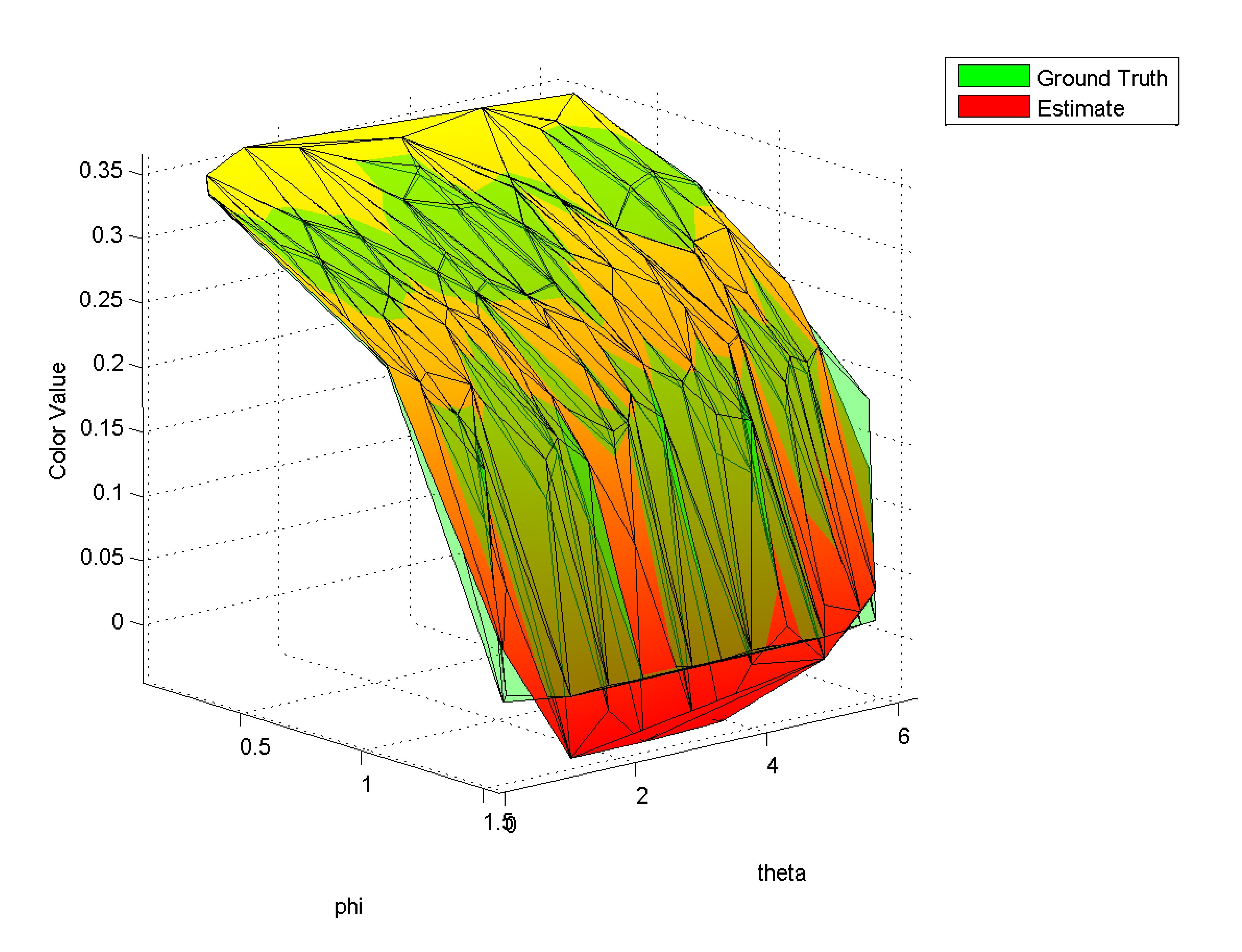
| Figure 4: Estimated color value and ground truth for a cube vertex of the scene in table 1. The fall off of the surface for increasing color values is caused by the cosine-term of the shading model. | |
 |
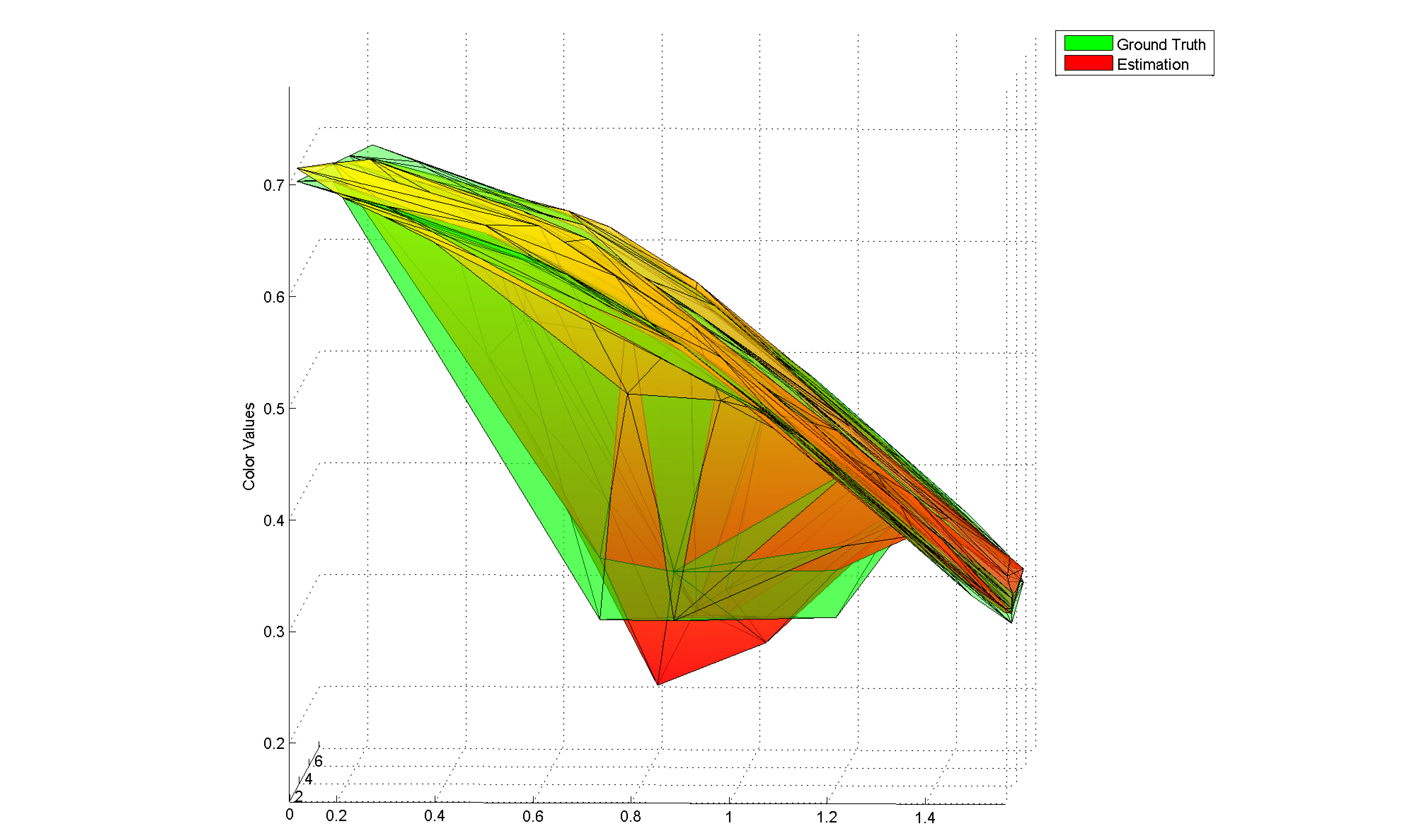 |
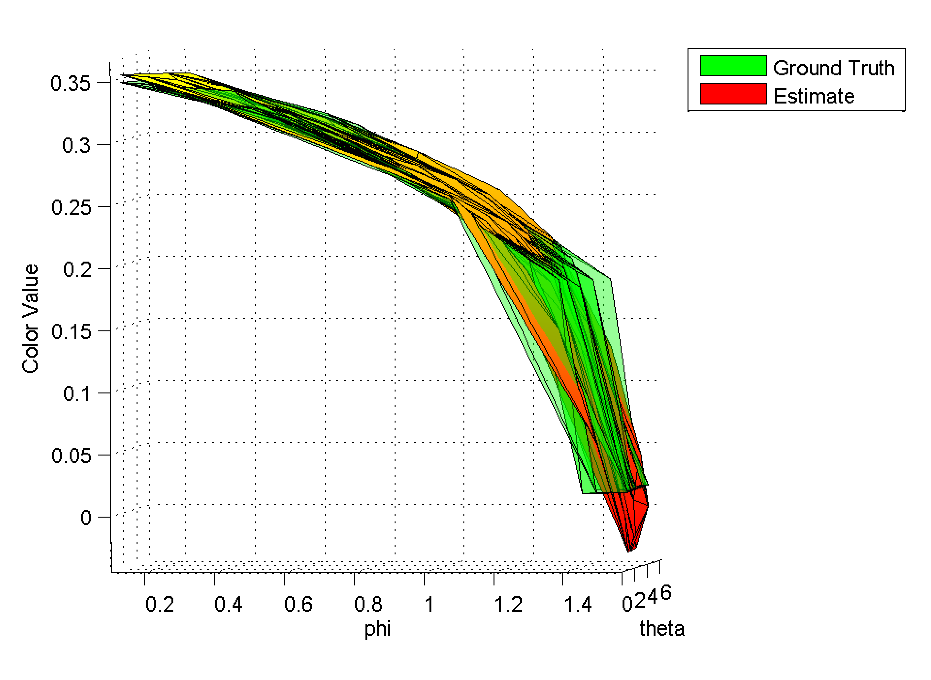
| Figure 5: Estimated color value and ground truth for a ground plane vertex of the scene in Figure 1. The fall off of the surface for increasing color values is caused by the cosine-term in the shading model. The valley is caused by the moving light so that a shadow occurs only for a certain view direction. | |
 |
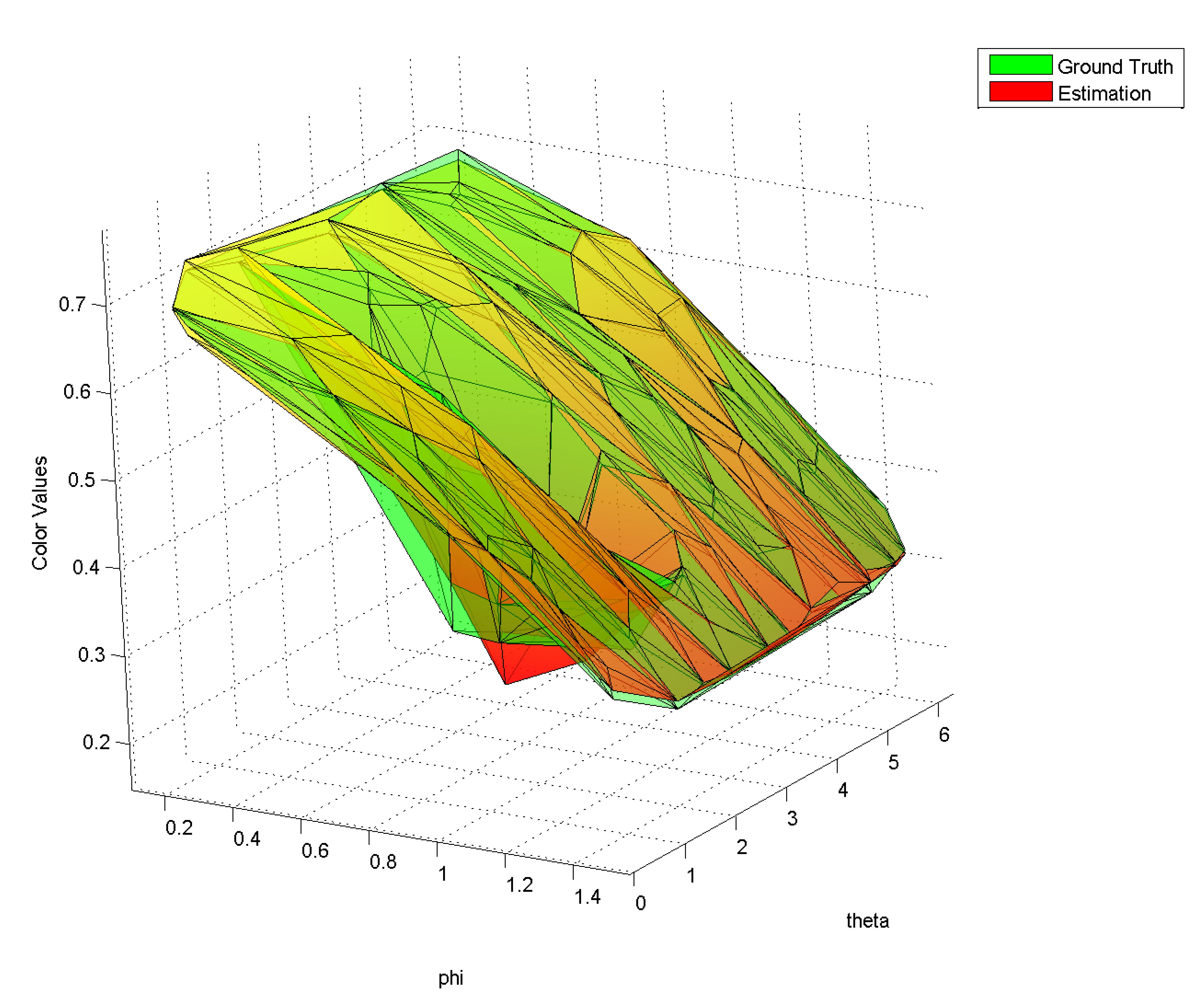
| Figure 3: Ground truth and estimated color value for the training data for one vertex in the ground plane in Figure 1. |
References:
- Arnold 1941
- K. J. Arnold, On spherical probability distributions, PhD Thesis (unpublished), Massachusetts Institute of Technology, 1941
- Bishop 1995
- C. M. Bishop, Neural Networks for Pattern Recognition, Oxford University Press, 1995
- Fisher 1987
- N. I. Fisher, Statistical analysis of spherical data, Cambridge University Press, 1987
- Gortler 1996
- S. J. Gortler, R. Grzeszczuk, R. Szeliski, M. Cohen, The Lumigraph, SIGGRAPH 1996, August 1996
- Green 2006
- P. Green, J. Kautz, W. Matusik, F. Durand, View-Dependent Precomputed Light Transport Using Nonlinear Gaussian Function Approximations, Proceedings of ACM 2006 Symposium in Interactive 3D Graphics and Games, 2006
- Hastie 2001
- T. Hastie, R. Tibshirani, J. Friedman, The Elements of Statistical Learning, Springer-Verlag, 2001
- Hillesland 2003
- K. E. Hillesland, S. Molinov, R.Grzeszczuk, Nonlinear optimization framework for image-based modeling on programmable graphics hardware, SIGGRAPH 2003, August 2003
- Jenison 1995
- R. Jenison, K. Fissell, A Comparison of the von Mises and Gaussian Basis Function for Approximating Spherical Acoustic Scatter, IEEE Transactions on Neural Networks, 6, 5, 1995, pp. 1284-1287
- Jenison 1996
- Rick L. Jenison and Kate Fissell, A Spherical Basis Function Neural Network for Modeling Auditory Space, Neural Computation, Vol. 8, Issue 1, pp. 115-128, January 1996
- MacRobert 1948
- T. MacRobert, Spherical harmonics; an elementary treatise on harmonic functions, with applications, Dover Publications, 1948
- Miller 1998
- G. Miller, S. Rubin, and D. Ponceleon, Lazy Decompression of Surface Light Fields for Precomputed Global Illumination, Eurographics Workshop on Rendering 1998, June 1998
- Orr 1998
- M. J. L. Orr, An EM algorithm for regularized RBF networks, International Conference on Neural Network and Brain, 1998
- Schröder 1995
- Peter Schröder, Wim Sweldens, Spherical wavelets: efficiently representing functions on the sphere, SIGGRAPH 1995, September 1995
- Ungar 1995
- L. Ungar, R. De Veaux, EMRBF: A statistical basis for using radial basis function for control, Proceedings of ACC 95, 1995
- Veach 1997
- Eric Veach, Robust Monte Carlo Methods for Light Transport Simulation, PhD dissertation, Stanford University, December 1997
- Wahba 1981
- G. Wahba, Spline interpolation and smoothing on the sphere, SIAM Journal on Scientific and Statistical Computing, 2, 5-16, 1981
- Wood 2000
- D. N. Wood, D. I. Azuma, K. Aldinger, B. Curless, T. Duchamp, D. H. Salesin, W. Stuetzle, Surface light fields for 3D photography, SIGGRAPH 2000, July 2000
- Zickler 2005
- T. Zickler, S. Enrique, R. Ramamoorthi, P. Belhumeur, Reflectance Sharing: Image-based Rendering from a Sparse Set of Images, Eurographics Symposium on Rendering. 2005, June 2005
| lessig (at) dgp.toronto.edu | 2005/12/22 |